Mutual Information and Diffusion Processes
A Collaborative Effort

Giulio Franzese
Eurecom

Pietro Michiardi
Eurecom
Mustapha Bounoua
Eurecom

Chao Wang
Eurecom
Alberto Foresti
Eurecom / Politecnico di Torino
Luca Nepote
Eurecom
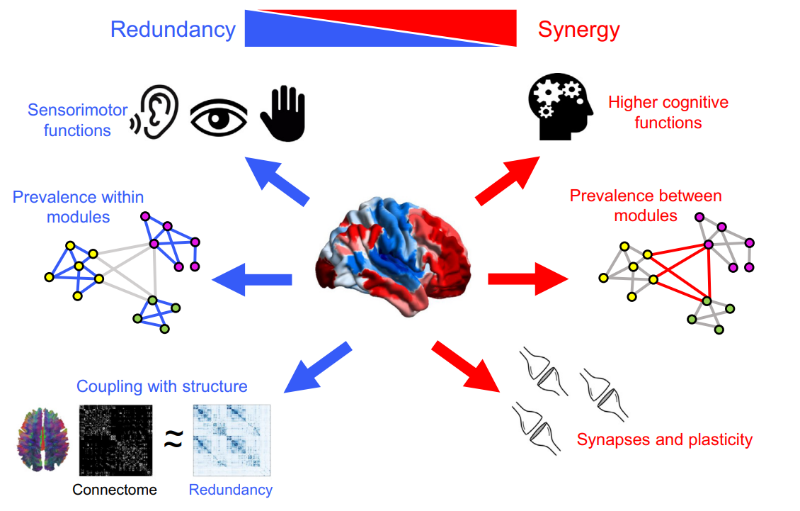
A Glimpse of What MI Can Reveal
One formula — five biological questions.
Mutual Information Estimators…? (cont.)
Discriminative approaches in one slide (convex duality of \(\phi(\cdot)\)):
\[\phi^{*}(y)=\sup_{x}(xy-\phi(x)),\quad \phi^{**}(x)= \sup_{y}(yx-\phi^{*}(y)),\quad \phi^{**}(x)=\phi(x)\]
Donsker-Varahdan Thm: \[\KL{\mu}{\chi}=\sup_{T:\Omega\rightarrow\mathbb{R}}\E_\mu[T]-\log \E_\chi [\exp(T)]\]
From all possible functions \(T\) to the smaller class of neural networks: \[\sup_{T:\Omega\rightarrow\mathbb{R}}(\E_\mu[T]-\log \E_\chi [\exp(T)])\geq \sup_{\theta\in \mathbb{R}^K}(\E_\mu[T^\theta]-\log \E_\chi [\exp(T^\theta)])\]
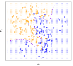
- Big problems: i) Good luck with MC estimation of \(\log \E [\exp(T^\theta)]\); ii) For tail events, estimation is unreliable.
The Diffusion Idea — An Intuition
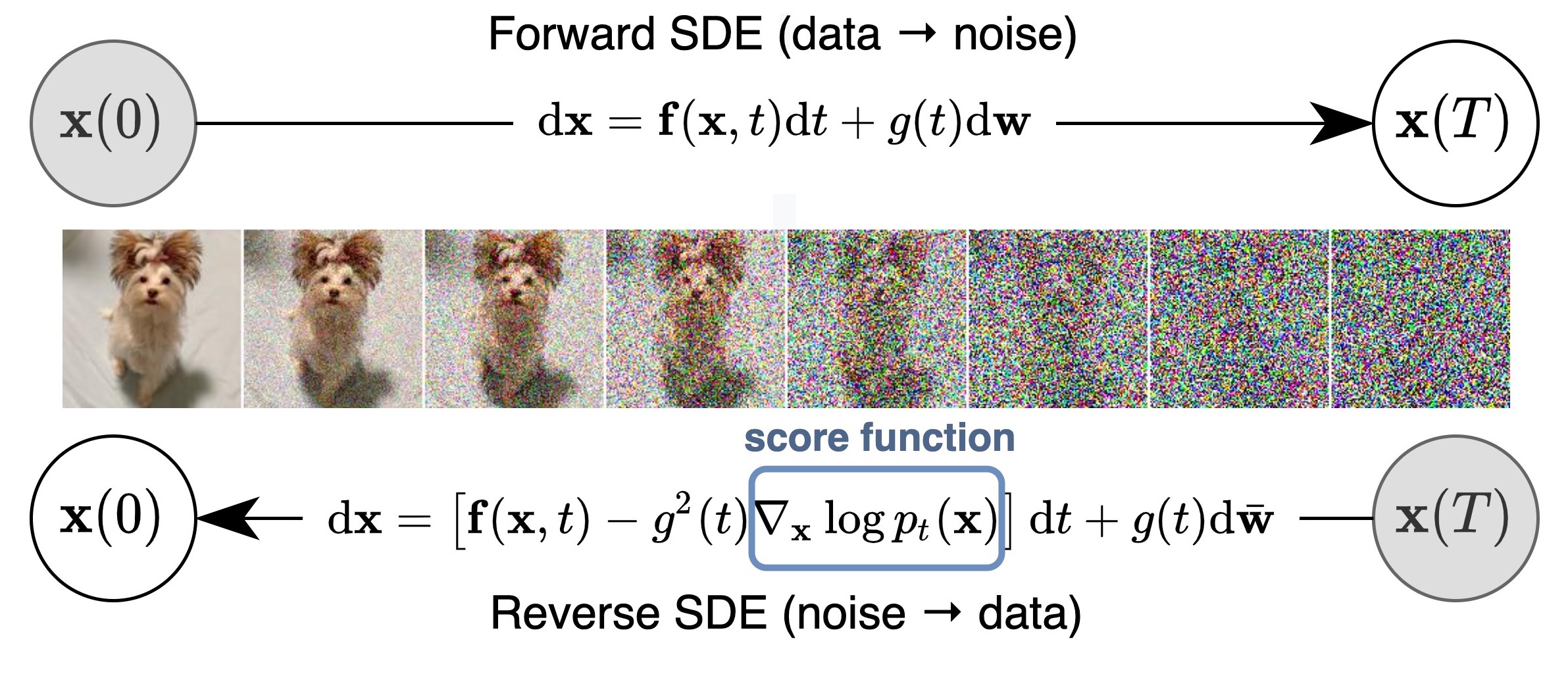
Step 1 — Forward process (noising):
Any distribution \(p(x)\) converges to a Gaussian when you repeatedly add small amounts of noise.
\[x_t = e^{-t}\,x_0 + \sqrt{1 - e^{-2t}}\;\varepsilon, \quad \varepsilon \sim \mathcal{N}(0,I)\]
- At \(t=0\): the original data distribution.
- At \(t\to\infty\): pure Gaussian noise.
- The trajectory in between is fully tractable.
Step 2 — Score function = compass toward data:
\[\nabla_x \log p_t(x) \;\;\text{"points toward high-density regions"}\]
- Intuitively: a noisy sample \(x_t\) “knows” where \(x_0\) came from.
- The score is proportional to the optimal denoiser (Tweedie’s formula):
\[\nabla_x \log p_t(x) = \frac{e^{-t}\,\mathbb{E}[x_0 \mid x_t] - x_t}{1 - e^{-2t}}\]

Step 3 — Learn the score, get MI for free:
Train a neural network to denoise (self-supervised): \[\mathcal{L}(\theta) = \mathbb{E}\!\left[\|\text{net}_\theta(x_t, t) - x_0\|^2\right]\]
The gap between two denoisers encodes the KL divergence — and therefore the Mutual Information.
Score-based Generative Models?
The time reversal of diffusion processes is currently one of the main ingredients behind the extremely popular generative AI models (Stable Diffusion, DALL·E, Sora…).
These models are trained to denoise — which means they implicitly learn the score \(\nabla \log p_t(x)\) at every noise level.
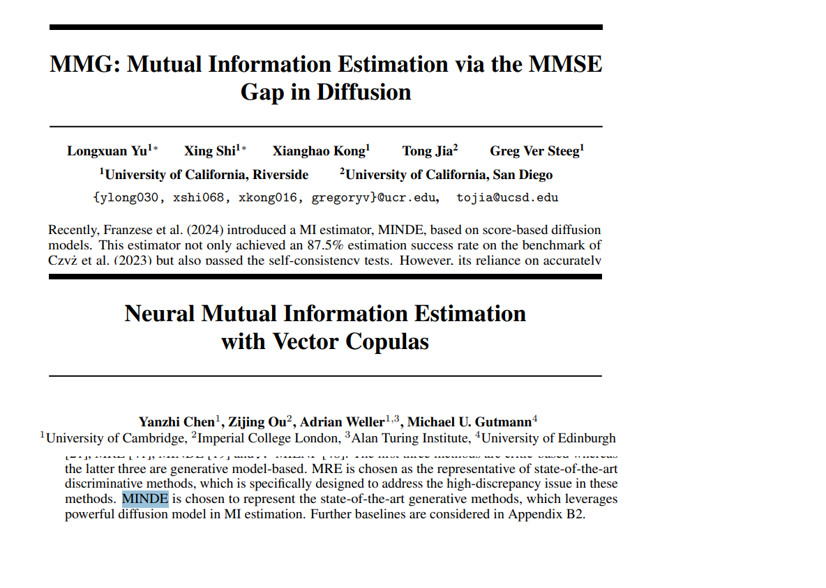
Mutual Information Neural Diffusion Estimation
Mutual Information between two random variables \(A,B\):
\[\textsc{I}(A,B)=\KL{\mu^{A,B}}{\mu^A\mu^B}\]
Two families of diffusion processes: joint (J) and conditional (C).
\[\begin{cases}\dd [X_t,Y_t]^\top =-[X_t,Y_t]^\top \dd t+ \sqrt{2}\,[\dd W_t,\dd W'_t]^\top\\ [X_0,Y_0]^\top\sim \mu^{A,B}\end{cases}\]
The joint and marginal scores are the only ingredients needed — train a single network, query it twice.
The Route Matters, Not Just the Endpoints
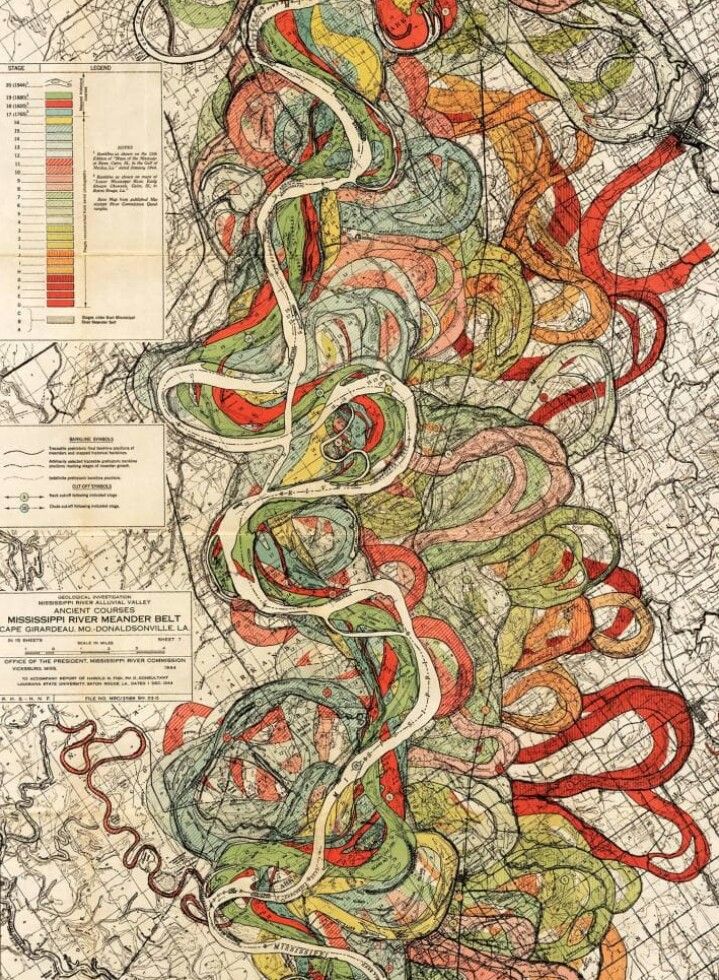
The Mississippi’s source and mouth are fixed — yet its path meanders unpredictably across thousands of miles.
In trajectory inference, we observe cell populations at a few snapshots. Standard metrics (W₂, MMD) compare those snapshots — but infinitely many paths connect the same marginals. The route is invisible to marginal metrics.
We need a metric defined on distributions over paths, not distributions at individual timepoints.
MINDE in Infinite Dimensions: Trajectory-Level KL
The single-cell trajectory problem
scRNA-seq gives population snapshots at a few timepoints — but not trajectories. Trajectory inference methods reconstruct full paths \(X_{[0,1]}\) from these snapshots.
The evaluation gap: standard metrics compare marginals only. Infinitely many path measures produce identical marginals.
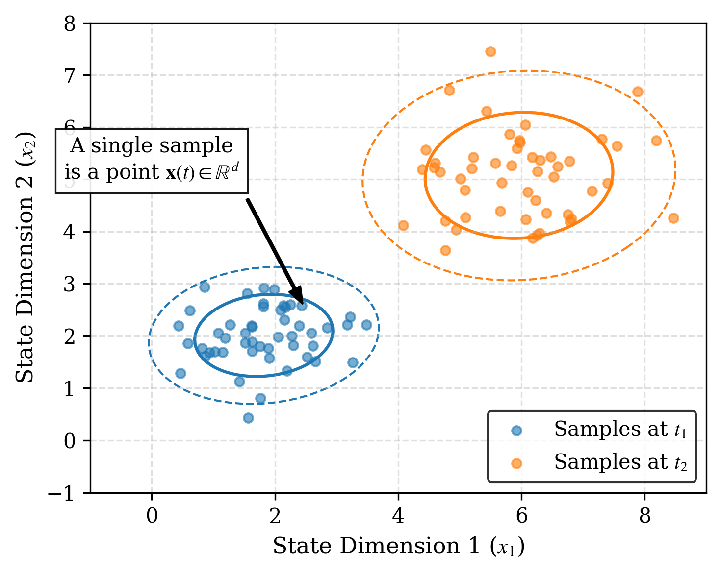
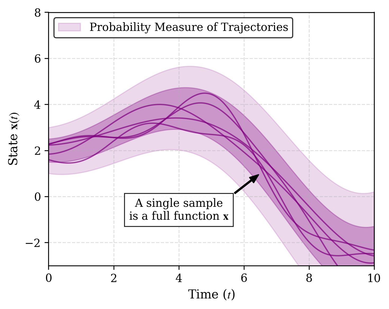
Trajectory KL Exposes What Marginal Metrics Miss
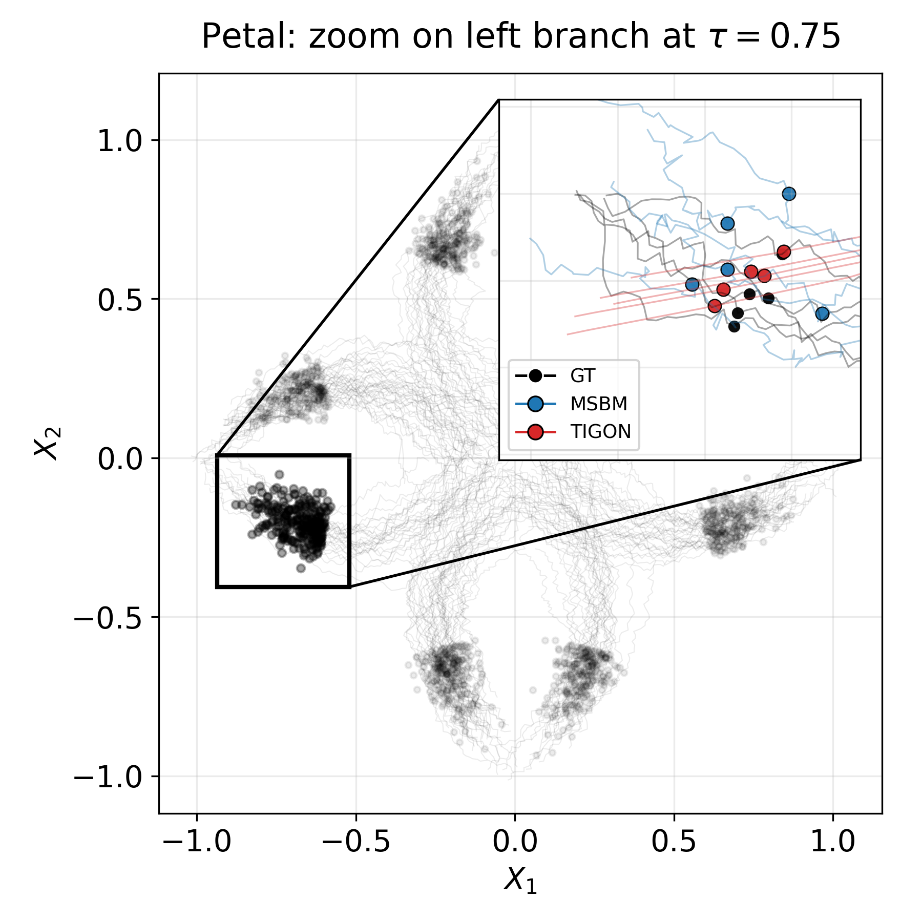
The petal dataset — a synthetic trajectory benchmark mimicking cell differentiation (branching, merging).
At \(\tau = 0.75\): MSBM and TIGON score nearly identically by Wasserstein distance (\(W_2 = 0.160\) vs \(0.155\)). Marginal metrics declare them equivalent.
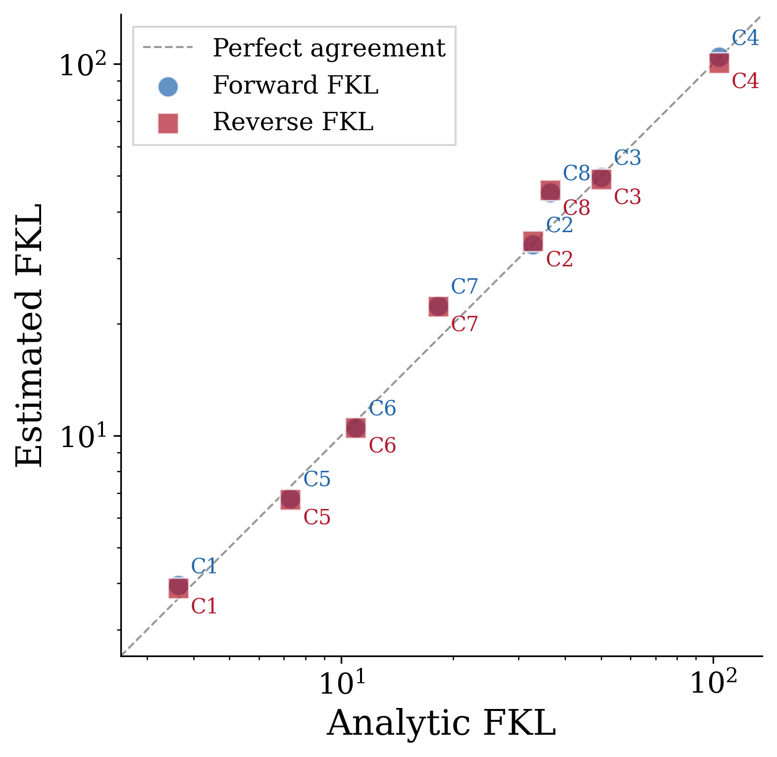
FKL correctly separates them — and is validated against analytical ground truth on Gaussian path measures:
Continuous Time Markov Chains (cont.)
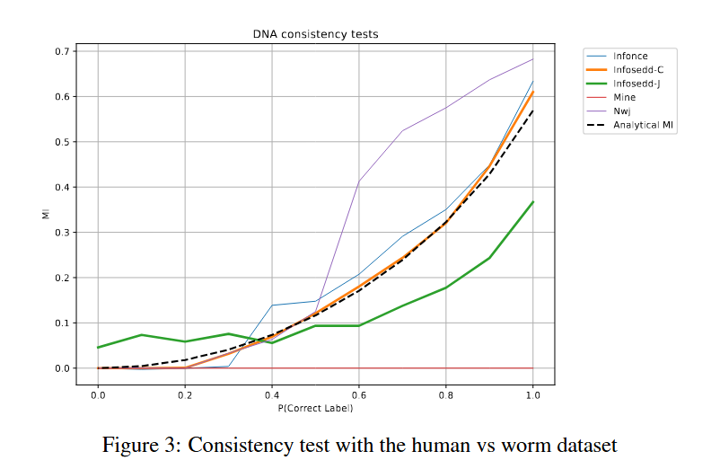
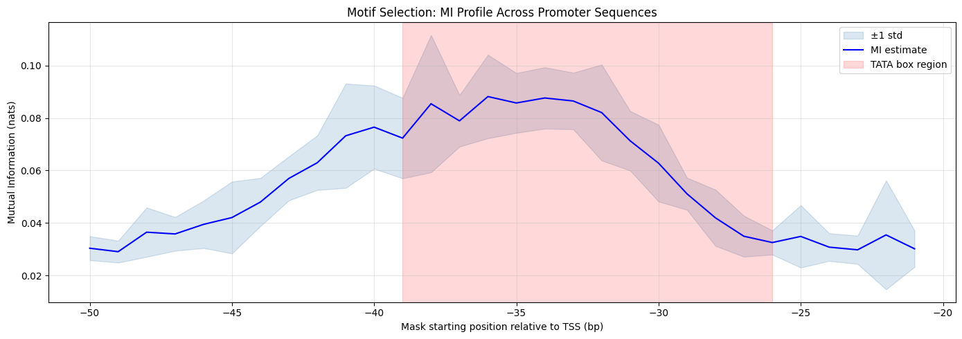
What MI is computed: \(I(\text{Window}_{[i,i+6)};\, \text{Label})\) — the information that a 6-bp DNA window carries about whether the sequence is a promoter or not. The window slides from −200 bp to +51 bp relative to the TSS.
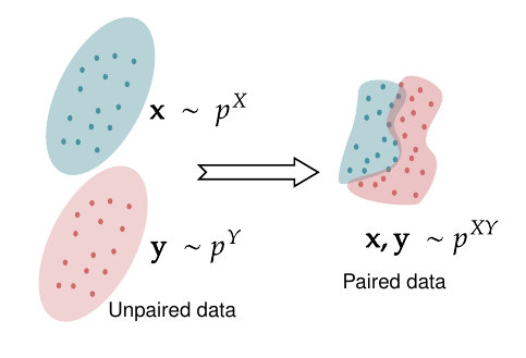
Unpaired Data Problem
- Multimodal learning often assumes the availability of paired data.
- However, real-world data is frequently unpaired across modalities.
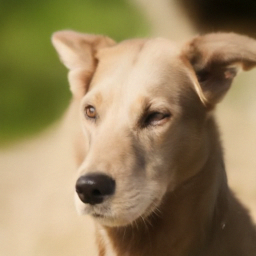
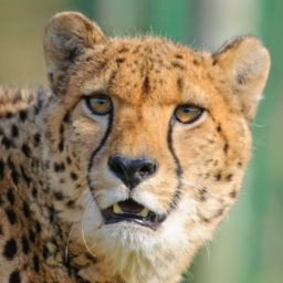
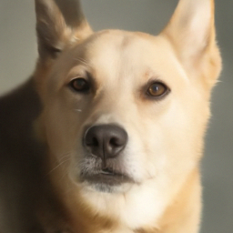
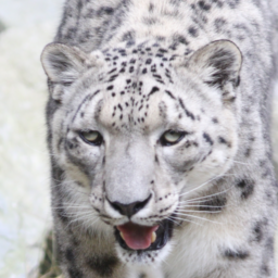
Unpaired Data: Demonstrated Results
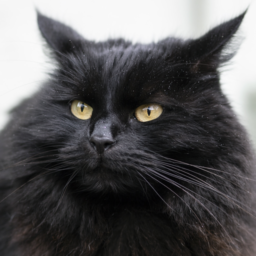
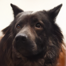
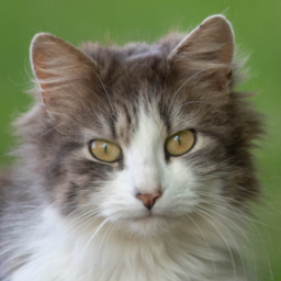
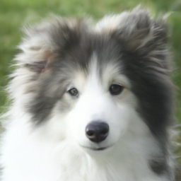
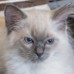
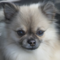
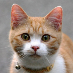
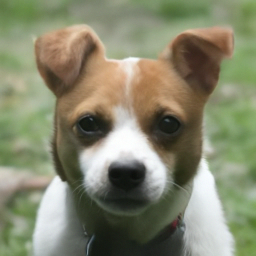
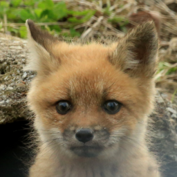
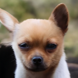
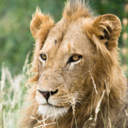
DDMEC can pair any two unpaired distributions — demonstrated on image domains:
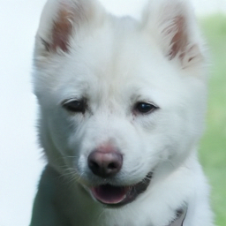
Unpaired Data: Application to Single-Cell Multi-Omics
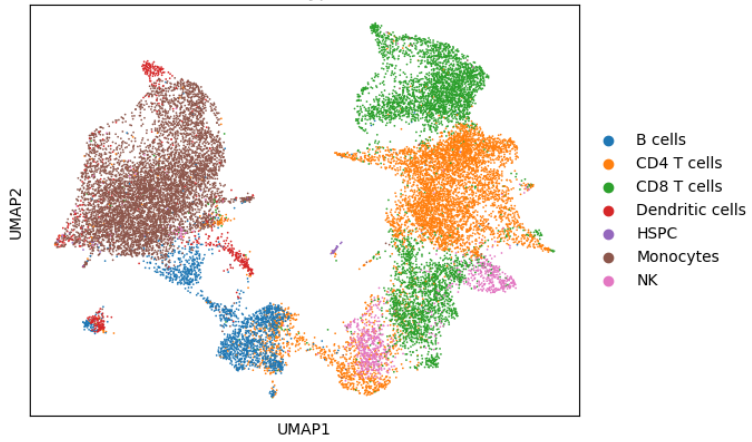
Application to single-cell multi-omics: aligning ATAC-seq (chromatin accessibility) with RNA-seq (gene expression) from the same cell population — without paired measurements.
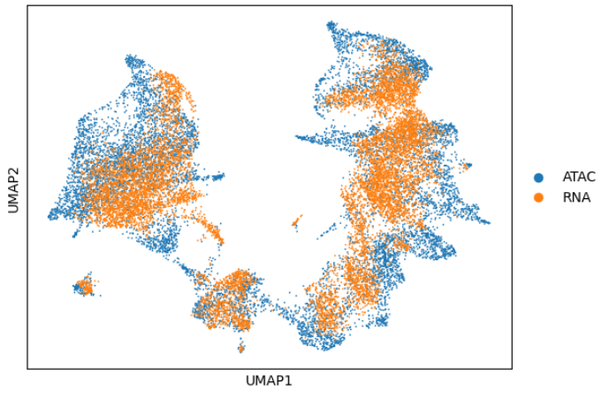
DDMEC demonstrated on PBMC single-cell data: joint chromatin + transcriptome alignment without paired profiling.
Multimodal Information Theory
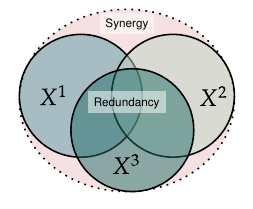
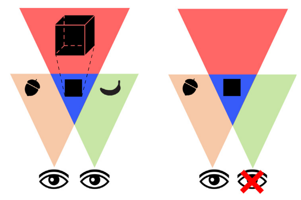
- Recently, the concept of MI has been extended to higher-order interactions: Redundant, Synergistic and Unique Information. Seminal works by Williams and Beer (Partial Information Decomposition). Extremely important in consciousness studies.
Multimodal Information Theory (cont.)
Applications: Multimodal sensory neuroscience.
O-Information
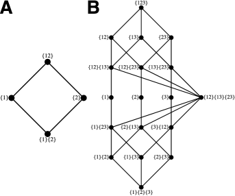
Analyzing systems with more than two variables. Example of metric: O-Information.
\[\Omega(X) = T(X) - D(X)\] where \(T(X) = \sum_{i=1}^{N} H(X_i) - H(X)\) is the Total Correlation and \(D(X) = H(X) - \sum_{i=1}^{N} H(X_i | X_{\backslash i})\) is the Dual Total Correlation.
- \(\Omega > 0\): redundancy dominates — each variable independently carries overlapping information
- \(\Omega < 0\): synergy dominates — variables jointly encode information no single one carries alone
Nice properties, but out of reach unless data are Gaussian (or “simple”) and/or discrete. The Hasse diagram (right) shows the full lattice of information atoms underlying the decomposition.
O-Information (cont.)
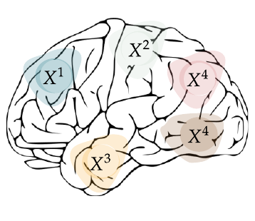
Real neural data does not follow a known parametric distribution. The marginal density of a single visual cortex area (right) is multimodal, skewed, and heavy-tailed.
Gaussian O-information estimators would be wrong by construction. A nonparametric, score-based approach is the only option that does not require assuming a distribution family.
Example: Analysis of Mice Brain Activity
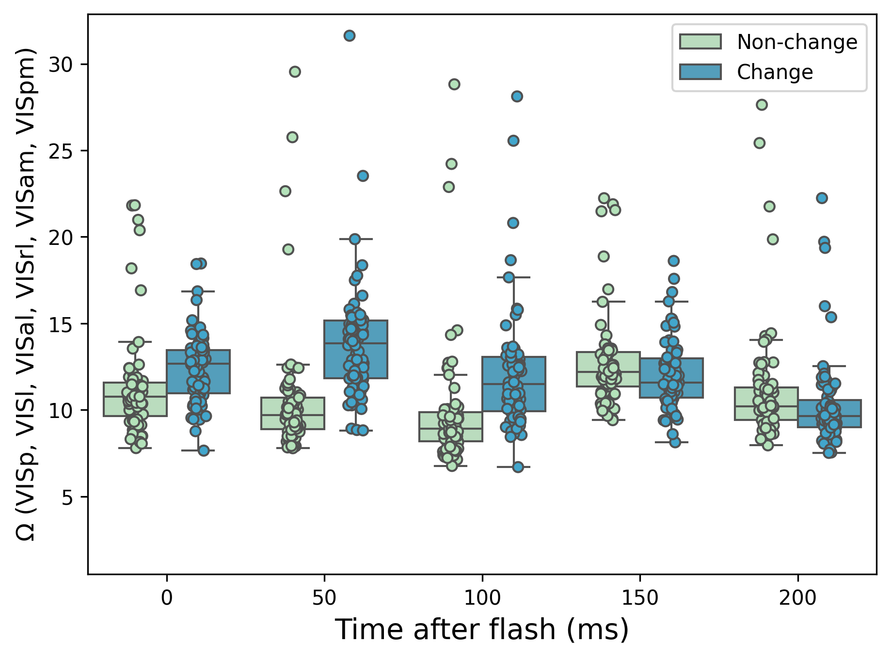
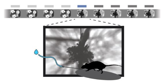
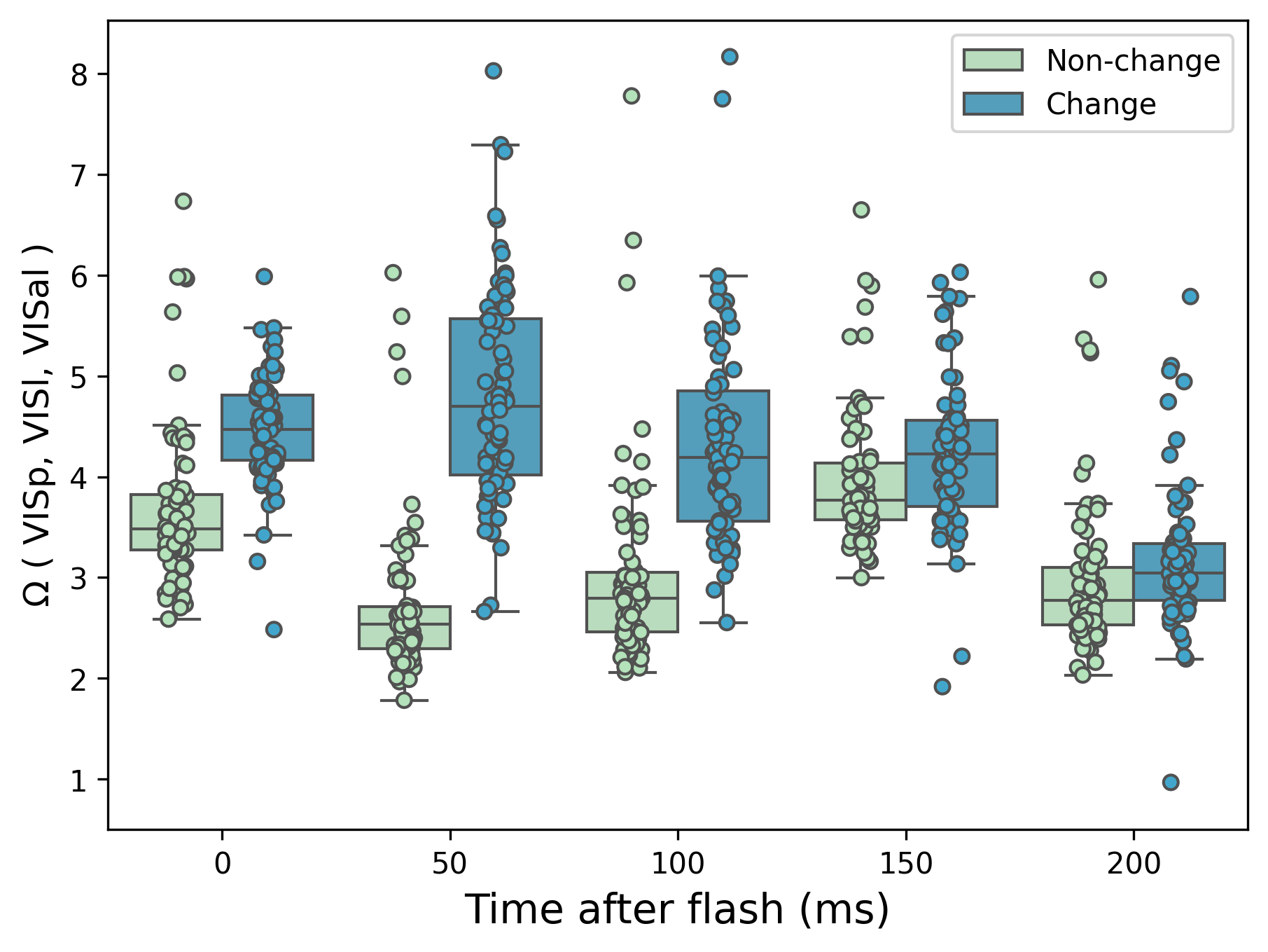
Quantity: \(\Omega(X_1,\ldots,X_6)\) where each \(X_i \in \mathbb{R}^5\) is the population response of one of 6 visual cortex areas recorded simultaneously via Neuropixels probes.
Areas: VISp (V1), VISl, VISal, VISrl, VISam, VISpm — 5 neurons × 6 areas = 30-dimensional joint response. Two conditions × 5 time bins after stimulus onset = 10 models.
- Novel stimulus (“change”) → \(\Omega > 0\) (redundancy): the joint response is statistically consistent with each area independently carrying overlapping information — one interpretation is redundant broadcast for reliability
- Repeated stimulus (“non-change”) → \(\Omega < 0\) (synergy): the joint response is statistically consistent with a shared code that no single area fully carries — one interpretation is efficient joint coding emerging with familiarity
What this unlocks: no previous estimator could compute O-information on 30-dimensional neural data. The score-based approach handles arbitrary distributions, revealing the redundancy→synergy transition that linear (Gaussian) estimators miss entirely.
Mice Brain Activity Results
TENDE: Example
Real physiological data: 10-minute recording (~6000 samples at ~10 Hz), z-score standardised.
Quantity computed: \(\mathrm{TE}_{\text{resp}\to\text{HR}}\) and \(\mathrm{TE}_{\text{HR}\to\text{resp}}\) for lags \(k \in \{2,4,6,8,10\}\) seconds.
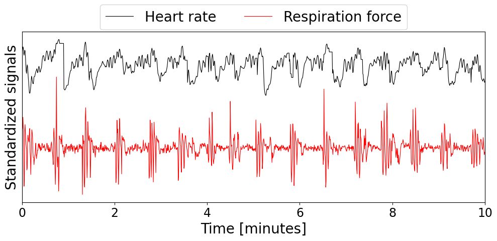
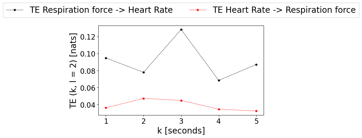
What is recovered: cardiorespiratory coupling — breathing modulates heart rate more than the reverse.
Application: Mosaic Brain Organoids
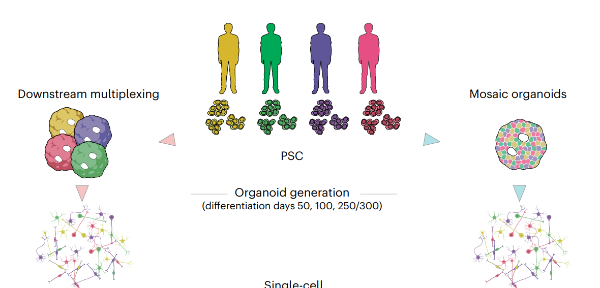
Caporale et al. (Nature Methods, 2024): multiplexing cortical brain organoids from multiple donors enables longitudinal dissection of developmental traits at single-cell resolution.
Co-cultured clonal lineages may depart from independent single-lineage behaviour — SOI and TENDE would allow us to test whether non-additive interactions shape clonal dynamics in ways that pairwise correlation cannot detect.
SOI and TENDE apply directly:
SOI — \(\Omega(\text{lineage}_1, \ldots, \text{lineage}_N)\): when does clonal co-culture switch from redundant (independent expansion) to synergistic (non-additive coordination)? The sign change is a quantitative marker of emergent interaction.
TENDE — \(\mathrm{TE}_{\text{lineage}_i \to \text{lineage}_j}(k)\): which lineage drives which, and when? Maps the causal structure of clonal dynamics as the mosaic matures.