Mutual Information and Diffusion Processes — Backup
Giulio Franzese — Eurecom, Data Science Department
An Informal Introduction
An informal introduction
Probability Spaces
- A probability space \((\Omega, \mathcal{F}, \mathrm{P})\) consists of:
- \(\Omega\): The sample space (set of all possible outcomes).
- \(\mathcal{F}\): A \(\sigma\)-algebra, a collection of subsets of \(\Omega\) representing events.
- \(\mathrm{P}\): A probability measure that assigns a number between 0 and 1 to each event in \(\mathcal{F}\).
Understanding \(\sigma\)-Algebra in Simple Terms
- A \(\sigma\)-algebra can be understood as defining the granularity of information available.
- It must satisfy:
- The whole sample space \(\Omega\) is included.
- If an event is in \(\mathcal{F}\), its complement must also be in \(\mathcal{F}\).
- If a countable sequence of events is in \(\mathcal{F}\), their union must also be in \(\mathcal{F}\).
- Example: Rolling a dice.
- \(\Omega = \{1,2,3,4,5,6\}\).
- A possible \(\sigma\)-algebra: \(\{\emptyset, \Omega, \{1,3,5\}, \{2,4,6\}\}\) (representing even and odd outcomes).
Understanding \(\sigma\)-Algebra (cont.)
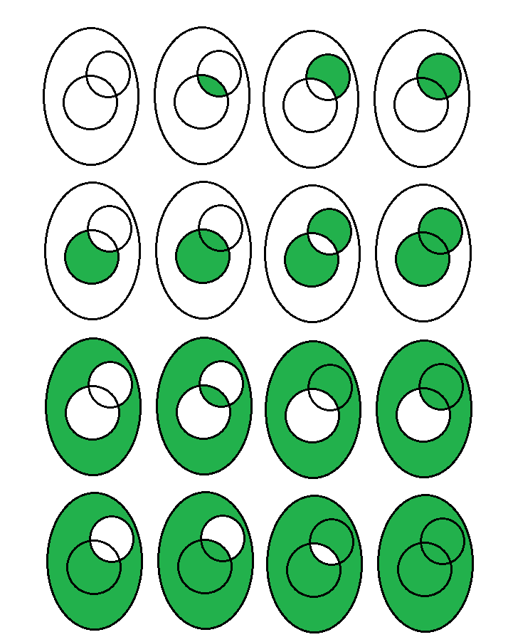
Example of \(\sigma\)-algebra
Random Variables as Mappings
- A random variable \(X\) is a function that maps outcomes from the sample space \(\Omega\) to real numbers: \[X: \Omega \to \mathbb{R}\]
- Example 1: Rolling a dice. If \(\omega\in\Omega=\{1,2,3,4,5,6\}\), then \(X(\omega)=\omega\).
- Example 2: Defining an odd/even variable. \(Y(\omega)=1\) if \(\omega\) is odd, \(Y(\omega)=0\) if \(\omega\) is even.
Random Variables as Mappings (cont.)
- A random variable must be measurable with respect to a given \(\sigma\)-algebra to be well-defined.
- Example:
- With \(\sigma\)-algebra \(\{\emptyset,\Omega,\{1,3,5\},\{2,4,6\}\}\), \(Y\) (odd/even) is measurable.
- However, \(X\) (exact roll outcome) is not measurable — a finer \(\sigma\)-algebra is needed.
- Intuitive interpretation: Doob’s lemma: A random variable is measurable with respect to a \(\sigma\)-algebra if and only if there exists a function that depends only on elements of the algebra.
Introduction to Stochastic Processes
- A stochastic process is a collection of random variables indexed by time: \[Y_t: \Omega \to \mathbb{R}, \quad t \geq 0\]
- It describes how a system evolves randomly over time.
- Examples:
- Stock prices.
- Population dynamics.
- Temperature variations.
Filtration and Adapted Processes
- A filtration is a sequence of \(\sigma\)-algebras representing growing information over time: \[\mathcal{F}_0 \subseteq \mathcal{F}_1 \subseteq \mathcal{F}_2 \subseteq \dots\]
- Intuitively, it models the accumulation of knowledge as time progresses.
- A process is adapted if at each time instant it is measurable with respect to the filtration.
Probability Measure
(Informal, not complete) In the framework of measure theory, a probability measure \(\mu\) is a mapping from subsets \(\{S_i\}_i\) of a given sample space \(\Omega\) such that:
- It is positive: \(\mu(S_i)\geq 0\)
- For disjoint sets \(S_i,S_j\) (\(S_i\cap S_j=\emptyset\)) it holds \(\mu(S_i\cup S_j)=\mu(S_i)+\mu(S_j)\).
- Its “integral” is equal to one: \(\mu(\Omega)=1\).
Familiar examples:
- \(\Omega=\mathbb{R}\), Gaussian probability \(\mu(dx)=p(x)dx=\frac{1}{\sqrt{2\pi}}\exp(-\frac{x^2}{2})dx\)
- \(\Omega=\{0,1\}\), Bernoulli RV \(\mu(\{0\})=\mu(\{1\})=\frac{1}{2}\)
Definition of SDEs
- A stochastic differential equation (SDE) is a particular class of stochastic processes.
- A general diffusion process on a probability space \((\Omega,\mathcal{F},\mathrm{P})\) is given by: \[Y_t(\omega) = Y_0(\omega) + \int_0^t H(Y_s(\omega),t)\,ds + W_t(\omega)\] where:
- \(Y_t\) is the stochastic process.
- \(H(Y_t(\omega),t)\) is the drift term.
- \(W_t\) is a Brownian motion, representing Gaussian noise.
- It only makes sense when considered with respect to a filtration \((\mathcal{F}_t)_{t\geq 0}\), representing the available information over time.
Formal MINDE Derivation
- Consider a probability space \((\Omega,\mathcal{F},\mathbb{P})\), together with a growing filtration \(\mathcal{F}_t\)
- Consider a generic random variable \(A\) (\(\mathcal{F}_0\)-measurable) with probability measure \(\mu^A(dx)\)
- Build a simple SDE in \([0,T]\) with initial conditions \(\sim\mu^A\): \[\begin{cases}\dd X_t=-X_t\,\dd t+\sqrt{2}\,\dd W_t,\\X_0=A\sim\mu^A\end{cases}\] where \(W_t\) is an \(\mathcal{F}_t\) Brownian motion.
- This SDE corresponds to a path measure \(\mathbb{P}^{A}\).
- Two SDEs which differ only by initial conditions have KL divergence: \[\KL{\mathbb{P}^{\mu^A}}{\mathbb{P}^{\mu^B}}=\E_{\mathbb{P}^{\mu^A}}\!\left[\log\frac{d\mathbb{P}^{\mu^A}}{d\mathbb{P}^{\mu^B}}\right]=\KL{\mu^A}{\mu^B}\]
Formal MINDE Derivation (cont.)
Time-reversal \(\hat{X}_t\defeq X_{T-t}\):
- KL is invariant to time-reversal: \(\KL{\mathbb{P}^{\mu^A}}{\mathbb{P}^{\mu^B}}=\KL{\hat{\mathbb{P}}^{\mu^A}}{\hat{\mathbb{P}}^{\mu^B}}\)
- Time reversal of SDE is again an SDE [Léonard 2014]
- Score function \(\leftrightarrow\) Denoiser (same as before)
Girsanov theorem:
\[\KL{\hat{\mathbb{P}}^{\mu^A}}{\hat{\mathbb{P}}^{\mu^B}}\simeq \E_{\mathbb{P}^{\mu^A}}\!\left[\int_0^T\norm{\nabla\log p^{A}_t(X_t)-\nabla\log p^{B}_t(X_t)}^2\dd t\right]\]
- Combining with time-reversal invariance → KL-estimator!
- Initial conditions \(\KL{\mu^A_T}{\mu^B_T}\) should be negligible (Bakry-Emery condition / ergodicity [Collet, Malrieu 2008])
Experimental Results
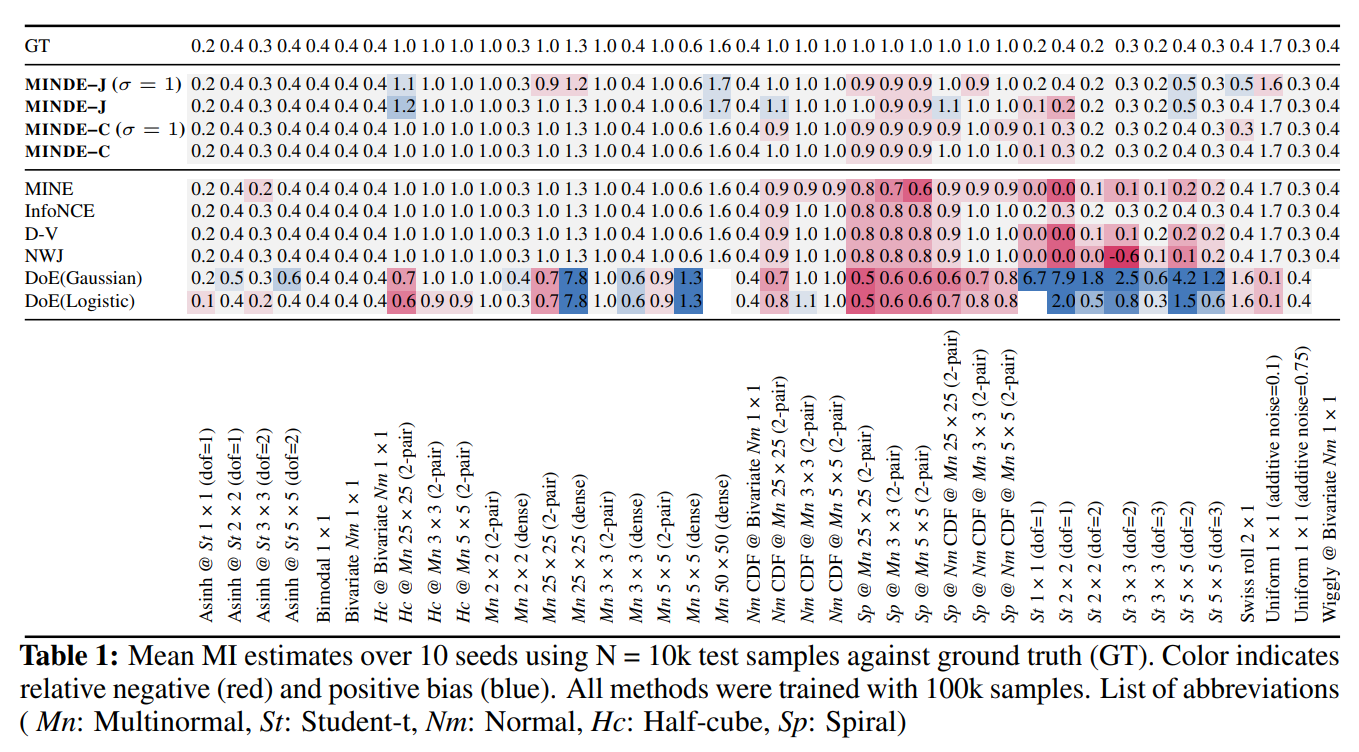
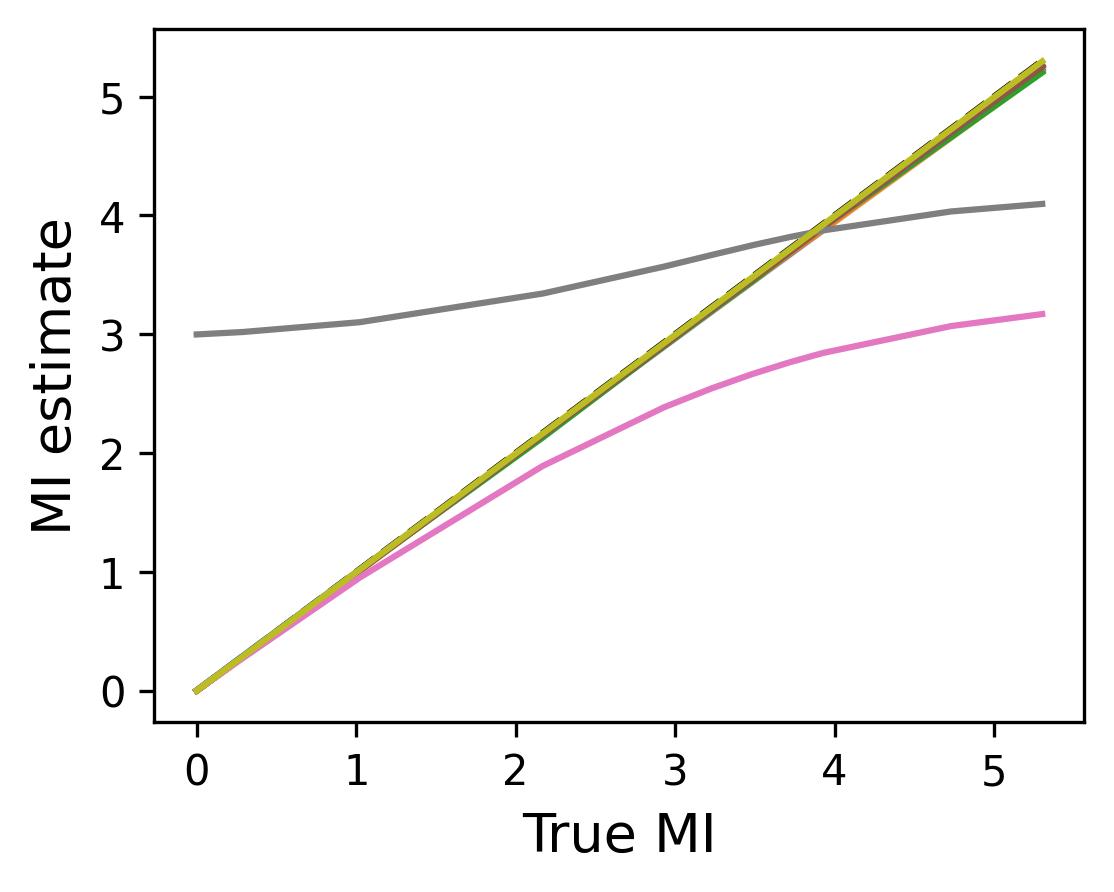
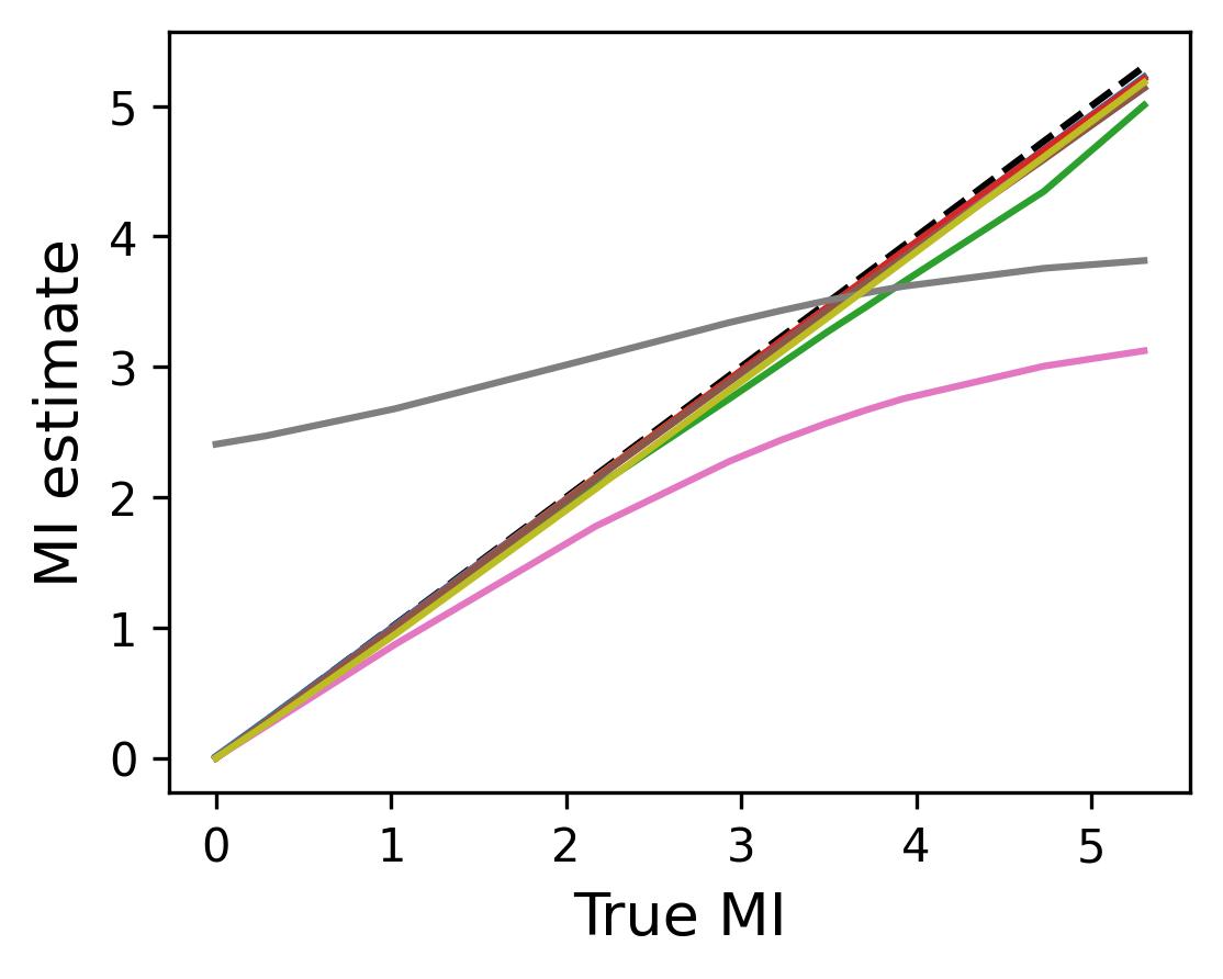
MINDE variants:
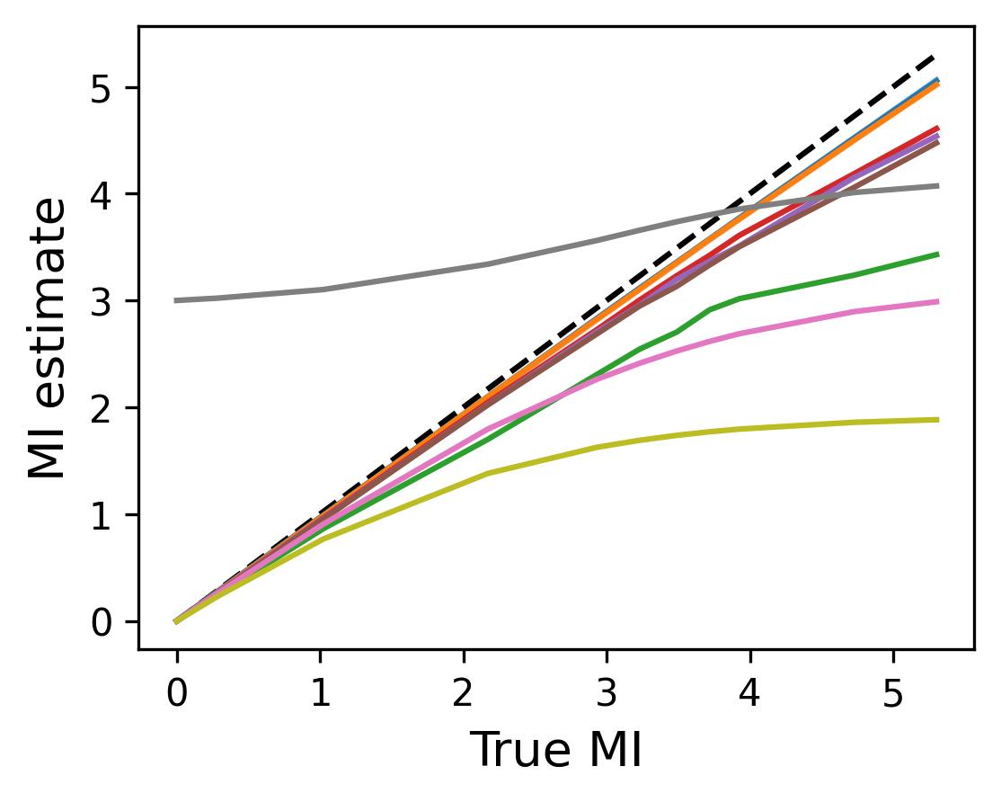
- Consistently outperform all competitors on standard benchmarks.
- Are capable of accurately estimating MI in the challenging High MI benchmarks:
Experimental Results (cont.)
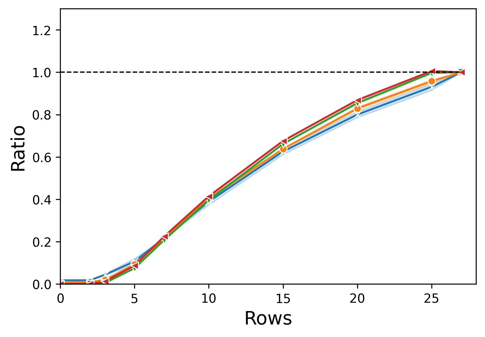
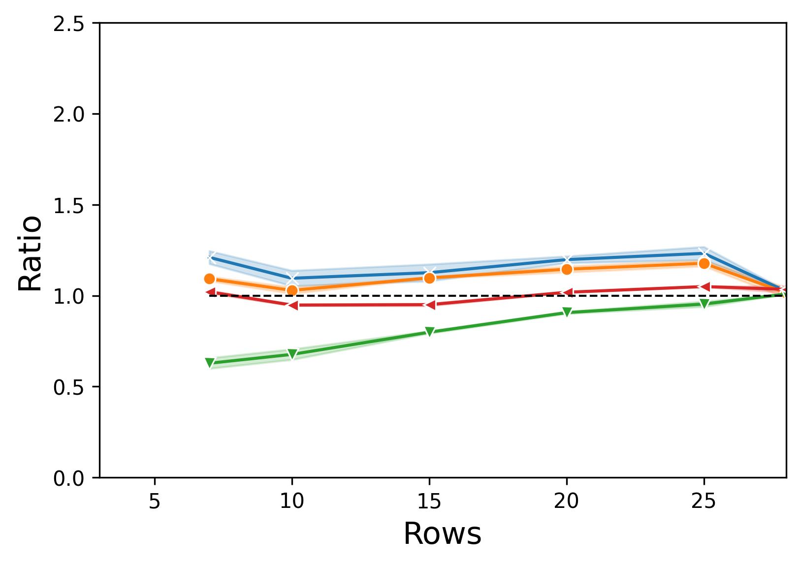
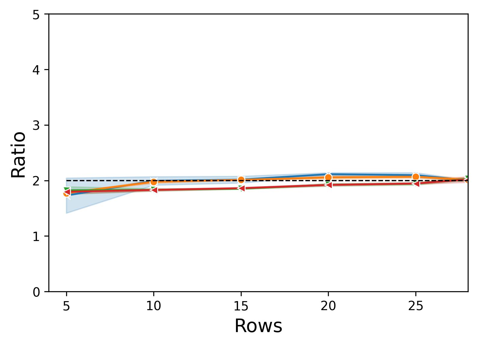
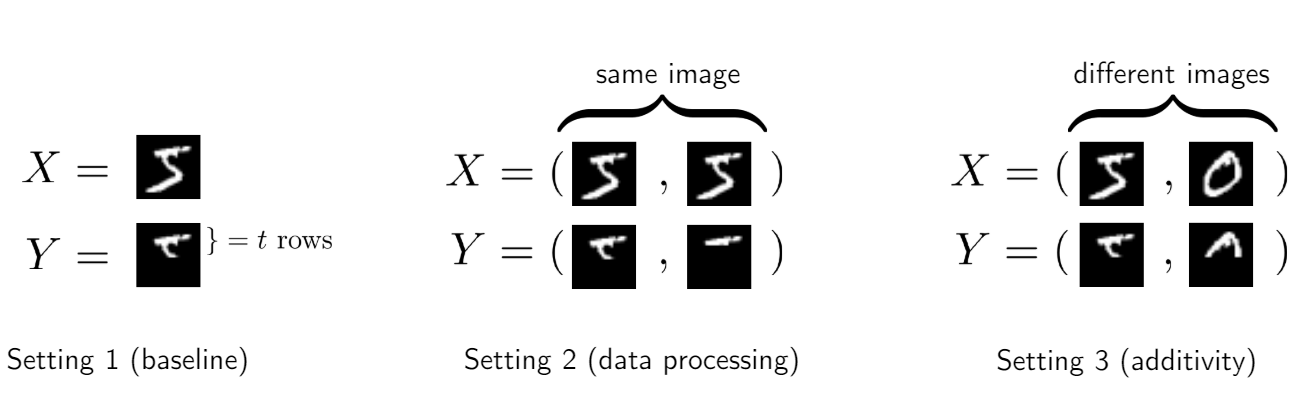
Pass the self-consistency tests: